October 2022, Vol. 249, No. 10

Features

Putting Machine Learning to Use for Integrity Management

By Jonathan Martin, Senior Data Scientist and Amine Ait Si Ali, Principal Data Scientist, ROSEN UK 

(P&GJ) — Minimizing the unscheduled downtime of a pipeline network is a crucial part of ensuring maximum throughput and therefore helping to ensure profitability. As an industry, we know that one of the best ways to achieve this is to develop and maintain an effective risk assessment and an associated integrity management plan, acting on the outcomes of them and ensuring we have a good understanding of the current condition of the pipeline and the rate at which it is deteriorating.   

There are, of course, several pipeline threats to consider, and operators use various technologies to monitor them. For a buried onshore pipeline, one of the key threats to maintaining the “original condition” of the pipeline is external corrosion, and an inline inspection (ILI) system will give a good idea of how external corrosion is currently affecting the pipeline. If the pipeline is re-inspected, estimates can then be made of the deterioration rate for different segments of the pipeline.  

Understanding where corrosion is growing is critical for ensuring reliability because it is typically growing defects that cause incidents, not stable anomalies. Identifying areas of active growth allows operators to act and prevent future incidents, delivering reliability.  

According to data compiled by the U.S. Department of Transportation’s (DOT’s) Pipeline and Hazardous Materials Safety Administration,¹ 8.1% of the pipeline incidents reported in the U.S. in 2021 were a result of external corrosion on the pipelines affected.   

This proportion increases to 11.2% when considering only those incidents classified as significant, qualified by the increased human, financial or environmental costs associated with the incident. Ensuring that the condition of a pipeline is well understood is paramount to ensuring that the risk of a significant incident is minimized.  

However, what if you cannot inspect your pipeline? Industry research suggests that many the world’s pipelines are difficult to inspect with conventional ILI tools and pipeline integrity engineers must therefore rely on alternative methods (e.g., external corrosion direct assessment [ECDA]) to maintain an acceptable understanding of a pipeline’s current condition and compliance with regulatory requirements.  

It is well understood that external corrosion initiates on a pipeline in corrosive environments that are coincident with external coating damage and ineffective cathodic protection (CP). As such, it is possible to describe the varying environment that the pipeline passes through using a series of parameters that could be considered to have an influence on the expected levels of external corrosion. These predictor variables include, but are certainly not limited to, the following:  

• External coating  
• Land use  
• Intersections (e.g., power lines, rail, road, etc.)   
• Age  
• Local rainfall  
• Soil type  

If the location of the pipeline right-of-way is known, then it is possible to gather information on the geospatial predictor variables from external data sets using a spatial join; this process is known as geo-enrichment. It can be performed for any pipeline where we have repeat ILI data. From that, we can generate a data model ion which there is a relationship between the predictor variables, the expected condition and the associated corrosion growth rates (CGRs).   

In short, if our data model contains sufficient quality and quantity of data to cover the predictor variable domain of our uninspected pipeline, we can infer CGR distributions along the length of the pipeline with reasonable confidence. This article describes the approach developed to calculate generalizable CGR parameters for use in a probabilistic assessment of pipelines where previous inspection data are either limited or not available.²  

The general approach takes the following steps:  

1. Perform anomaly matching for each repeat inspection in the data set and calculate CGRs for each anomaly, assuming linear growth between each inspection. Assign the relevant predictor variables to each anomaly (i.e., perform geo-enrichment).  
2. Segment the matched external corrosion anomalies into clusters, across the full data set, so that each cluster can be explained by their associated predictor variables.   
3. For each cluster identified, fit an appropriate distribution to the calculated CGRs in the cluster, extracting the associated distribution parameters.  
4. For the uninspected pipeline, generate the required predictor variables for the given pipeline route (if the length of each pipe spool is unknown, a standard interval can be assumed).  
5. For each pipe spool in the uninspected pipeline, determine the most similar cluster from the data set of inspected pipelines, and therefore CGR distribution parameters, based on their associated predictor variables.  
6. Use these distribution parameters as an input to assist in probabilistic integrity assessments.  

As an asset integrity company with decades of ILI data, collected from tens of thousands of pipelines across the globe, ROSEN is in a position to generate insights (on a macro level) into how both the condition and observed deterioration of those assets correlate with the metadata collected about them. To support this endeavor, ROSEN has developed the Integrity Data Warehouse (IDW), a database containing ILI data aligned with additional pipeline integrity-related data sources.  

The process described hereafter follows from a study of determining CGR distributions from about 244,000 pipeline spools (from 66 repeat inspections of pipelines located in North America), where geo-enrichment had been performed. Forty clusters were identified as part of this study where CGR distribution parameters could be provided, and the clusters could be clearly explained through certain characteristics of their predictor variables. This would allow, if all required metadata were collected, for varying CGR distributions to be selected for an uninspected pipeline.  

Dimensionality Reduction  

Experience tells us that external CGRs can be affected by many factors. This is partly because there are multiple corrosion mechanisms that may be active (for example, microbially induced corrosion, stray current corrosion or differential aeration corrosion).   

These different mechanisms are influenced by factors such as soil type, coating condition (in some cases a few small coating defects may have worse effects than many larger areas of degraded coating), rainfall, grown water level, etc.   

Consequently, we require a means to simplify the data set. Dimensionality reduction is the process of transforming data from a high-dimensional to a low-dimensional space (i.e., 2-D or 3-D) while retaining as much of the variance contained in the data as possible. We are then able to cluster the data in this low-dimensional space but retain the ability to explain each cluster using all available predictor variables.  

There are various methods to perform dimensionality reduction, each with their appropriate applications. The data set is both complex and non-linear in nature, requiring a method that can handle the complexity without being too computationally expensive. For that reason, we selected UMAP (uniform manifold approximation and projection).³   

This method fits a manifold to the data, which is necessary to capture the non-linearity of the data set. It also retains more of the global structure of the data compared with some of the other manifold learning methods (i.e., we retain the separation between data points that are dissimilar to one another in the high-dimensional space when we convert it to the low-dimensional space).   

Selection of appropriate hyperparameters (the variables that control how the dimension reduction method works) allowed for the data set to be reduced from 21 dimensions to 3.  

Our data set contains discrete categorical descriptors among the predictor variables; therefore, it is necessary to convert these into a numerical representation of their relationship with each other. A naïve approach to this would be to equally distribute the descriptors in the range from zero to one.   

However, it is possible to encode the predictor variables in such a way as to represent how a subject matter expert would consider their effect on the target variable (e.g., we could engineer an additional soil-type feature considering how well a given soil drains water, encoding sand as 1 and clay as 0.    

Segmentation  

To fit probability distributions to the calculated CGRs, it is necessary to determine which of the data points are closely associated (in terms of their predictor variables) with one another.   

With the data set reduced to a lower-dimensional space, it is possible to visualize and cluster the data more easily. Considering the data in terms of clusters helps us to get an understanding of what predictor variables are driving the similarities between pipeline spools in the entire data set. For example, one cluster could span multiple pipelines, defined by the soil type histosols, with a construction date in the 1970s.  

Provided enough data points, the CGR probability distribution could be calculated and described in terms of those predictor variables. Without the ability to call on unsupervised clustering techniques, it would be exceedingly difficult to capture the presence of such a cluster, let alone when also considering the relevance of the other predictor variables.  

Density-based clustering (examples include DBSCAN⁴ and OPTICS⁵) is often considered more appropriate for complex data sets because it can find arbitrarily shaped clusters based on density, rather than distance, between two points. These methods generate a fixed number of clusters based on the defined model parameters.  

Computation expense is another concern, given the iterative nature of this work. Therefore, as part of this work, consideration was also given to a hierarchical clustering technique called BIRCH.⁶ This algorithm is very memory-efficient and does not require each clustering decision to access all the other data points. (Figure 1)

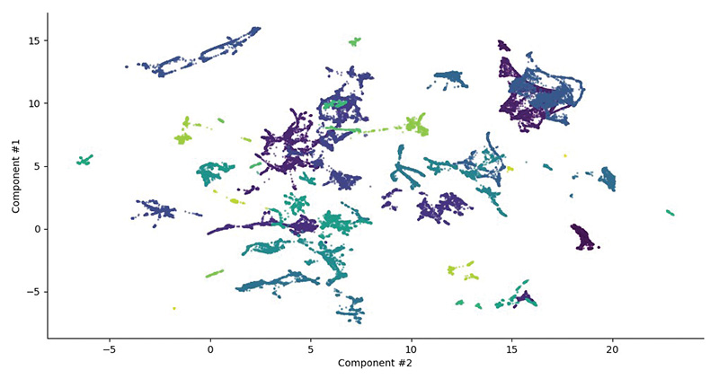
Although the density-based clustering algorithms took longer to compute, OPTICS was the clustering method that was chosen given the noticeable improvement it gave in explaining as many of the clusters identified as possible. Figure 1 shows how the clusters vary across the UMAP decision space. If the number of records, or number of predictor variables, were to increase, then it would be expected that the performance of the BIRCH would make it the more favorable clustering technique.  

Distribution Fitting  

Determining statistical distribution parameters to be used as part of a probabilistic risk assessment requires both the most appropriate statistical distribution to be selected and the error between the real data set and the theoretical distribution to be minimized.   

This process was carried out using Python’s SciPy package. This package determines the maximum likelihood estimate (MLE) for the distribution parameters that best represent the population sample. There are multiple methods of validating fitted distributions and, in this case, we used the Kolmogorov-Smirnov (K-S) test statistic. The best-fit distribution will result in the smallest K-S test statistic value.  

The parameters and distribution selected can also be verified using a visual verification of the empirical cumulative density function (CDF) against the simulated CDF. In our study, the statistical distributions selected included normal, log normal and Weibull.   

Care should be taken when using a normal distribution because it extends to negative infinity and truncation is required when it is included in a probabilistic assessment (this is to negate the physical impossibility of negative CGRs).  

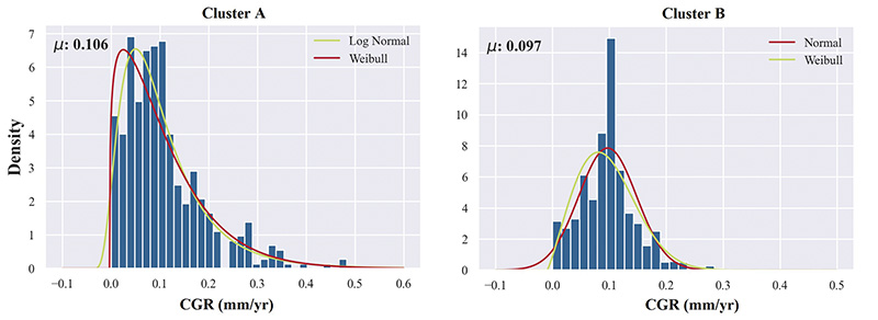
Figure 2 gives an example of two clusters that were identified following dimensionality reduction with both a Log Normal and Weibull distribution fitted to the matched external CGRs for Cluster A. The matched external CGRs for Cluster B, on the other hand, follow more of a symmetrical distribution and a Normal distribution and Weibull distribution were, therefore, selected.

Cluster Selection  

For a pipeline spool from an uninspected pipeline where we have both the geo-enriched and additional construction metadata, we need to identify the best match from the set of clusters that we have generated. To do this, it is necessary to reduce the number of dimensions representing the pipeline spool using the UMAP dimensionality reduction technique, using the model fitted to the training data set.   

With a reduced number of dimensions, we can then very simply identify the cluster considered closest in terms of their UMAP components. Taking the average cluster ID assigned to the nearest data points could also be considered. This would help justify the cluster selection when the UMAP transformation leaves the data point on the edge of a cluster.  

The process was followed for a test pipeline that was also in a similar location to those used to generate the 40 clusters shown in Figure 1, ensuring that the domain space is as similar as possible.   

As an example, a spool was chosen from the pipeline route and the most appropriate cluster identified from the model. This cluster represented matched external corrosion anomalies from three different pipelines, covering 665 pipe joints with similar associated properties, including:  

• Spool age of about 40 years  
• Podzol soil type (characterized by high pH and aerobic conditions)  
• High average annual rainfall  

The matching cluster has an average CGR of 0.1 mm/year where a Weibull distribution (β = 1.266, η = 4.54, γ = −0.12) was chosen (Cluster A in Figure 2).  

Conclusion  

This work has shown that realistic external CGR distributions can be generated using a machine learning model for pipelines that have not been inspected. These CGRs vary along the length of the pipeline and will identify those locations where the highest growth rates can be expected. This will give operators a clearer understanding of risk, and the ability to plan mitigation.  

Further Work  

The process described here demonstrates how statistical distribution parameters can be generated to represent the external CGRs that are observed in a network of pipelines, given a range of metadata (both construction and geospatial related), and how this information can be used to select the parameters for a pipeline we are unable to inspect.   

Predicting the future condition of a pipeline depends on more than the rate at which it is currently deteriorating; we also need to determine the expected current condition. Therefore, it is necessary that a model to determine both the likelihood of a given location having external corrosion present and the depth at which it is likely to be, should precede this process.  

Further to that, the study consisted of repeat ILIs for 66 pipelines in North America. To create a series of cluster types that can be generalized for external corrosion distributions across most buried pipeline environments, it is necessary to increase the number of pipelines substantially.   

It is expected that this will bring challenges on the computing side of things, and we will be required to produce further novel ways of handling such complexity.   

References:  

_{[1] Pipeline and Hazardous Materials Safety Administration. 2021. “Pipeline Incident 20 Year Trends.” Accessed August 8, 2022. https://www.phmsa.dot.gov/data-and-statistics/pipeline/pipeline-incident-20-year-trends.} 

_{2 Carrell, S., J. White, K. Taylor, J. Martin, S. Irvine, and R. Palmer-Jones. 2022. “Predicting External Corrosion Growth Rate Distributions for Onshore Pipelines for Input into Probabilistic Integrity Assessments.” The Digital Pipeline Solutions Forum 2022, May 2022.} 

_{[3] McInnes, Leland, John Healy, and James Melville. 2018. “Umap: Uniform manifold approximation and projection for dimension reduction.”} 

_{[4] Ester, Martin, Hans-Peter Kriegel, Jörg Sander, and Xiaowei Xu. 1996. „A density-based algorithm for discovering clusters in large spatial databases with noise.” In Proceedings of the Second International Conference on Knowledge Discovery and Data Mining (KDD’96). AAAI Press, 226–231.} 

_{[5] Ankerst, M., M.M. Breunig, H.-P. Kriegel, and Jörg Sander. 1999. “Optics: Ordering points to identify the clustering structure.” ACM Sigmod Record 28(2): 49–60.} 

_{[6] Zhang, T., R. Ramakrishnan, and M. Livny. 1996. “Birch: an efficient data clustering method for very large databases.” ACM Sigmod Record 25(2): 103–114.} 

Related Articles