
October 2024, Vol. 251, No. 10
Features
Risk Assessment: Comprehensive Review Concerning Rehab Analysis
By Eduardo Munoz, Principal Consultant, Dynamic Risk
Editor’s note: This is the first of a two-part article. Part 2 will appear in the October edition of P&GJ.
(P&GJ) — Risk models are prominent pipeline integrity management (PIM) tools used to make data-driven decisions. As computing power has increased and data acquisition methods have proliferated, risk models have become more complex.
Moreover, the transition to quantitative risk assessment (QRA) techniques and the heightened intricacy of the corresponding risk models requires a greater amount of specific high-quality information to be provided as inputs for the risk models, including meta data generated during their production.
The PIM personnel is not necessarily informed on the information requirements. Therefore, a good understanding of the effect of data uncertainty upon the risk model results is crucial to apply the model effectively and ethically in any decision-making process.
In the United States, 49 CFR 192.917(4)c [1] specifies the implementation of a sensitivity analysis (SA) on the factors used to characterize both the likelihood and consequence of failure for gas pipelines.
Sensitivity Analysis
One way to conduct sensitivity analysis (SA) is to vary one input parameter of the model at a time while holding the others constant. This is arguably the simplest SA approach available for deterministic models, but it is not fit for probabilistic models.
The nominal values of the input parameters are often used for this type of one-at-a-time (OAT) sampling. The extreme values of the distribution are one of the most common ways to determine the sampling points of interest, although there are many more possibilities.
The most basic form of LSA involves determining the linear correlation between two variables: an input [Equation] and an output [Equation] derived from data that is quasi-randomly sampled [9]. The idea is to approximate the full risk model with a linear surrogate, i.e. [Equation].
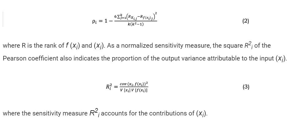
Pearson’s correlation coefficient (Equation 1) is the covariance of the two variables divided by the product of their standard deviations. The widely used Pearson correlation coefficient, Spearman rank correlation coefficient, and Partial correlation coefficient are typical local sensitivity methods.
The Pearson correlation coefficient is symmetric. A key mathematical property of the Pearson correlation coefficient is that it is invariant under separate changes in location and scale in the two variables.

LSA(b): Spearman rank correlation coefficients
In contrast to the Pearson correlation coefficient, the Spearman rank correlation coefficient, shown in Equation 2, imposes less stringent data condition requirements. A correlation between the observed values of the two variables is sufficient, or a monotonic relationship derived from a substantial quantity of continuous data is sufficient, irrespective of the two variables.
LSA(c): Partial correlation coefficients
A partial correlation coefficient is utilized to assess the degree of dependence between two variables in a population or data set that contains more than two characteristics. This strength of dependence is not considered when both variables change in response to variations in a subset of the other variables. Therefore, the Partial Correlation Coefficient (PCC) is the correlation coefficient where the linear effect of the other terms is removed, i.e. for [Equation] we have:

The result of correlation coefficient indices is a number between –1 and 1 that measures the strength and direction of the relationship between two variables. As with covariance itself, the measure can only reflect a linear correlation of variables and ignores many other types of relationships or correlations. The method demonstrates a comparatively low computational cost that is nearly unaffected by the number of inputs. The quantity of model iterations necessary to achieve satisfactory statistical accuracy is model-dependent.
Global sensitivity analysis (GSA) techniques
GSA(a): Morris Method: The Morris Method employs finite difference approximations for SA and operates on the principle that estimating derivatives by moving in one dimension at a time and using sufficiently large steps can yield robust contributions to the overall sensitivity measurement. The procedure involves:
- Selecting a random starting point in the input space.
- Choosing a random direction and altering only the corresponding variable by [Equation].
- Estimating the derivative based on this single-variable perturbation and repeating the process.
Continuing this process through numerous iterations allows the mean of these derivative estimates to serve as a global sensitivity index. This approach enhances computational efficiency by utilizing each simulation for dual derivative estimates, offering a more resourceful alternative to other methods.
While it focuses on average changes rather than dissecting total variance, its computational advantage is compelling for preliminary global sensitivity assessments.
To refine the Morris Method for practical applications, certain adjustments are necessary. It is important to account for the potential nullification of positive and negative changes, which suggests the use of absolute or squared differences for a more accurate variance measure.
Moreover, it’s critical to ensure comprehensive exploration of the input space. This can be achieved by defining the distance between trajectories as the cumulative geometric distance between corresponding point pairs. By generating an excess number of trajectories and selecting those with the greatest distances, the method attains a broad coverage of the input domain.
When the implementation and computational cost of a model is high, the relative affordability of this technique makes it a viable option for conducting SA.
GSA(b): Derivative-based global sensitivity measures (DGSM)
To surpass the limitations of a linear model, successive linearization may be desired. Given that derivatives involve linearization, it is possible to evaluate derivatives on an average.
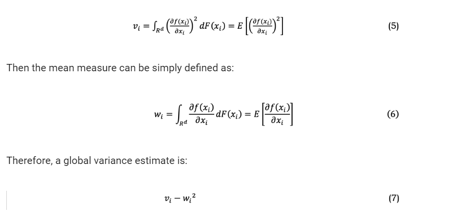
The Morris OAT sensitivity measure is contingent upon a nominal point [Equation]and it varies in response to a change in [Equation]. To address this inefficiency, one can calculate the average of [Equation] across the parameter space which is a unit hypercube [Equation]. Therefore, new sensitivity measures known as Derivative-based Global Sensitivity Measures (DGSM) can be defined.
Consider a function [Equation], where [Equation] are independent random variables, defined in the Euclidian space [Equation] , with cumulative density functions (CDF) of [Equation]. The following DGSM was introduced[20].
GSA(c-1): Variance-based methods: Sobol method
Variance-based approaches rely on the premise, proposed by Saltelli et al., [17], that the variance alone is enough to characterize the uncertainty of the output. Variance-based GSA techniques determine the effect on model outcome as a function of an appropriate parameter probability density function by decomposing the uncertainty of outputs for the corresponding inputs.
Sobol’s method [21] is a genuine technique for nonlinear decomposition of variance, making it highly regarded as one of the most reliable approaches. The approach partitions the variance in the system’s or model’s output into fractions that can be allocated to individual inputs or clusters of inputs.
First order and total order effects are the two primary sensitivity measures used in this method. The first order effects consider the primary effects for variations in output caused by the respective input. The total order effects represent the total contributions to the output variance related to the corresponding input, which include both first order and higher order effects owing to interactions between inputs.
The objective is to represent the output variance as a finite sum of elements that are arranged in ascending order. Each of the terms denotes the proportion of the output variance attributable to one input variable (first order terms) or the interaction variance of multiple input variables (higher order terms).
Subsequently, the Sobol’s sensitivity indices are established by normalizing these partial variances by the output variance.
GSA(c-2): Variance-based methods: FAST and eFAST methods
Two widely used and well-established GSA methodologies are the Fourier Amplitude Sensitivity Test (FAST) and the extended FAST (eFAST) which are faster ways of estimating the total order sensitivity indices [17,22].
The FAST method modified Sobol method allowing faster convergence. The FAST method allocates the variance through spectral analysis, following which the input space is explored with sinusoidal functions of varying frequencies for each input factor or dimension [10,14,17].
FAST transforms the variables [Equation] onto the space [0,1]. Then, instead of the linear decomposition, it decomposes into a Fourier basis:
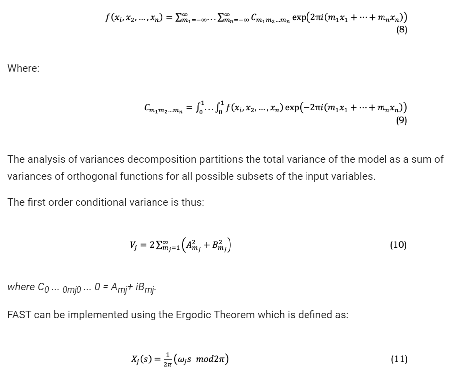
According to the Ergodic theorem, if [Equation] are irrational numbers, the dynamical system will not repeat values and will thus provide a solution that is densely distributed across the search space. This means that the multidimensional integral can be approximated by the integral over a single line.
One can approximate this to obtain a more simplified expression for the integral. By considering [Equation] as integers, it can be observed that the integral is periodic. Therefore, it is sufficient to integrate throughout the interval of 2π.
A longer period yields a more accurate representation of the space and hence a more precise approximation, while potentially necessitating a greater number of data points. Nevertheless, this conversion simplifies the genuine integrals into straightforward one-dimensional quadrature that may be effectively calculated.
To obtain the total index using this approach, it is necessary to compute the total contribution of the complementary set, denoted as [Equation], and subsequently:

It is important to note that this is a rapid method to calculate the overall impact of each variable, encompassing all higher-order nonlinear interactions, all derived from one-dimensional integrals. The extension is referred to as eFAST which is highly regarded in many scenarios due to several notable strengths:
- Handling non-linear and non-additive models: eFAST is particularly effective in analysing complex models with non-linear or non-additive effects. It can capture both the main effects and the interaction effects among input variables.
- Global SA: as a GSA method, eFAST evaluates the entire input space, as opposed to local methods that analyse sensitivity at a specific point in the input space. This comprehensive approach allows eFAST to provide more robust and generalizable insights.
- Frequency domain analysis: eFAST operates in the frequency domain, using Fourier transforms to decompose the model output into frequency components. This allows it to distinguish between the effects of different input variables based on their unique frequency signatures.
- Efficiency in handling many input variables: eFAST is more computationally efficient compared to some other global methods, particularly when dealing with a large number of input variables. This is due to its use of spectral decomposition, which can efficiently separate the effects of each input variable.
- Improved accuracy over FAST: eFAST extends the original FAST method by incorporating a wider range of frequency harmonics, allowing for the detection of higher-order interactions between variables. This leads to improved accuracy in the sensitivity estimates.
- Capability to identify non-linear interactions: eFAST is adept at identifying non-linear interactions between input variables, a crucial aspect for many complex systems where such interactions are significant.
GSA(d): Density-Based Methods
Density-based GSA methods compute the sensitivity of the inputs and their interactions by considering the complete probability density function (PDF) of the model output.
Their popularity stems from the fact that density-based SA methods can circumvent certain restrictions associated with interpreting variance-based measures when model input dependencies are present. Nevertheless, in situations involving a substantial number of model inputs (high dimensionality) or computation times of the model or function exceeding a few minutes, their estimation may become impracticable.
Two Density-based GSA methods are DELTA [23] and PAWN [24]. The DELTA (δ) approach is a density-based SA method that is not influenced by the method used to generate the samples. This method calculates the first order sensitivity and the δ (similar to total sensitivity) for each input parameter. DELTA tries to evaluate the impact of the entire input distribution on the complete output distribution, without considering any specific point of the output.
PAWN is called after the authors and its purpose is to calculate Density-based SA metrics in a more efficient manner. The main concept is to define output distributions based on their Cumulative Distribution Functions, which are simpler to calculate compared to Probability Density Functions.
One benefit of using PAWN is the ability to calculate sensitivity indices not only for the entire range of output fluctuation, but also for a specific sub-range. This is particularly valuable in scenarios when there is a specific area of the output distribution that is of interest.
Sampling strategies and Monte Carlo simulation
It is important to observe that each expectation involves an integral, so the variance is defined as integrals of integrals, which makes this computation quite complex. Therefore, Monte Carlo estimators are frequently employed. Instead of only relying on a pure Monte Carlo approach, it is common practice to employ a low-discrepancy sequence, which is a type of quasi-Monte Carlo method, to efficiently sample the search space.
There are two primary categories of structures for low discrepancy point sets and sequences: lattices and digital nets/sequences. For additional information on these constructions and their attributes, refer to [25]. Sobol sequences [26] are commonly employed as specific instances of quasi-random (or low discrepancy) sequences of a given size.
The low-discrepancy characteristics of Sobol’ sequences deteriorate as the dimension of the input space increases. The rate of convergence is adversely impacted if the crucial inputs are situated in the final components of inputs. Consequently, if there is an initial ranking of inputs based on their relevance, it would be advantageous to sample the inputs in decreasing order of importance to improve the convergence of sensitivity estimates.
The Latin Hypercube sampling (LHS) is another frequently used quasi-Monte Carlo sequence that extends the concept of the Latin Square. In the Latin Hypercube, only one point is assigned in each row, column, and so on, resulting in a uniform distribution across a space with multiple dimensions.
(Editor’s Note: Part 2 of this article will be published in the November issue of P&GJ)
This paper was originally presented at Clarion’s Pipeline Pigging Integrity Management Conference 2024.
References
[1] Pipeline and Hazardous Materials Safety Administration (PHMSA), RIN 2137–AF39 Pipeline Safety: Safety of Gas Transmission Pipelines: Repair Criteria, Integrity Management Improvements, Cathodic Protection, Management of Change, and Other Related Amendments, 2022. https://www.federalregister.gov/documents/2022/08/24/2022-17031/pipeline-safety-safety-of-gas-transmission-pipelines-repair-criteria-integrity-management (accessed December 2, 2023).
[2] M. Ionescu-Bujor, D.G. Cacuci, A Comparative Review of Sensitivity and Uncertainty Analysis of Large-Scale Systems—I: Deterministic Methods, Nuclear Science and Engineering 147 (2004) 189–203. https://doi.org/10.13182/NSE03-105CR.
[3] A. Ahmadi-Javid, S.H. Fateminia, H.G. Gemünden, A Method for Risk Response Planning in Project Portfolio Management, Project Management Journal 51 (2020) 77–95. https://doi.org/10.1177/8756972819866577.
[4] S.H. Fateminia, N.G. Seresht, A.R. Fayek, Evaluating Risk Response Strategies on Construction Projects Using a Fuzzy Rule-Based System, in: Proceedings of the 36th International Symposium on Automation and Robotics in Construction, ISARC 2019, 2019: pp. 282–288. https://doi.org/10.22260/ISARC2019/0038.
[5] S.H. Fateminia, P.H.D. Nguyen, A.R. Fayek, An Adaptive Hybrid Model for Determining Subjective Causal Relationships in Fuzzy System Dynamics Models for Analyzing Construction Risks, CivilEng 2 (2021) 747–764.
[6] S.H. Fateminia, A.R. Fayek, Hybrid fuzzy arithmetic-based model for determining contingency reserve, Autom Constr 151 (2023) 104858. https://doi.org/https://doi.org/10.1016/j.autcon.2023.104858.
[7] S.H. ‘Fateminia, Determining and Managing Contingency Reserve throughout the Lifecycle of Construction Projects, PhD Thesis, University of Alberta, 2023.
[8] A. Saltelli, K. Aleksankina, W. Becker, P. Fennell, F. Ferretti, N. Holst, S. Li, Q. Wu, Why so many published sensitivity analyses are false: A systematic review of sensitivity analysis practices, Environmental Modelling & Software 114 (2019) 29–39. https://doi.org/https://doi.org/10.1016/j.envsoft.2019.01.012.
[9] A. Saltelli, R. Marco, A. Terry, C. Francesca, C. Jessica, G. Debora, S. Michaela, T. Stefano, Global Sensitivity Analysis: The Primer, in 2008. https://api.semanticscholar.org/CorpusID:115957810.
[10] R. Ghanem, D. Higdon, H. Owhadi, Handbook of uncertainty quantification, Springer, 2017.
[11] S.H. Fateminia, V. Sumati, A.R. Fayek, An Interval Type-2 Fuzzy Risk Analysis Model (IT2FRAM) for Determining Construction Project Contingency Reserve, Algorithms 13 (2020) 163. https://doi.org/10.3390/a13070163.
[12] S.H. Fateminia, N.B. Siraj, A.R. Fayek, A. Johnston, Determining Project Contingency Reserve Using a Fuzzy Arithmetic-Based Risk Analysis Method, in: Proceedings of the 53rd Hawaii International Conference on System Sciences, Hawaii International Conference on System Sciences, 2020. https://doi.org/10.24251/hicss.2020.214.
[13] S. Razavi, A. Jakeman, A. Saltelli, C. Prieur, B. Iooss, E. Borgonovo, E. Plischke, S. Lo Piano, T. Iwanaga, W. Becker, The future of sensitivity analysis: An essential discipline for systems modeling and policy support, Environmental Modelling & Software 137 (2021) 104954.
[14] E. Borgonovo, G.E. Apostolakis, S. Tarantola, A. Saltelli, Comparison of global sensitivity analysis techniques and importance measures in PSA, Reliab Eng Syst Saf 79 (2003) 175–185. https://doi.org/https://doi.org/10.1016/S0951-8320(02)00228-4.
[15] E. Borgonovo, E. Plischke, Sensitivity analysis: A review of recent advances, Eur J Oper Res 248 (2016) 869–887. https://doi.org/https://doi.org/10.1016/j.ejor.2015.06.032.
[16] D.G. Cacuci, M. Ionescu-Bujor, A Comparative Review of Sensitivity and Uncertainty Analysis of Large-Scale Systems—II: Statistical Methods, Nuclear Science and Engineering 147 (2004) 204–217. https://doi.org/10.13182/04-54CR.
[17] A. Saltelli, R. Marco, A. Terry, C. Francesca, C. Jessica, G. Debora, S. Michaela, T. Stefano, Global Sensitivity Analysis: The Primer, in 2008. https://api.semanticscholar.org/CorpusID:115957810.
[18] C. Xu, G.Z. Gertner, Uncertainty and sensitivity analysis for models with correlated parameters, Reliab Eng Syst Saf 93 (2008) 1563–1573. https://doi.org/https://doi.org/10.1016/j.ress.2007.06.003.
[19] E. Borgonovo, Sensitivity Analysis, in: Tutorials in Operations Research: Advancing the Frontiers of OR/MS: From Methodologies to Applications, INFORMS, 2023: pp. 52–81. https://doi.org/doi:10.1287/educ.2023.0259.
[20] I.M. Sobol’, S. Kucherenko, Derivative based global sensitivity measures and their link with global sensitivity indices, Math Comput Simul 79 (2009) 3009–3017. https://doi.org/https://doi.org/10.1016/j.matcom.2009.01.023.
[21] I.M. Sobol′, Global sensitivity indices for nonlinear mathematical models and their Monte Carlo estimates, Math Comput Simul 55 (2001) 271–280. https://doi.org/https://doi.org/10.1016/S0378-4754(00)00270-6.
[22] R.I. Cukier, C.M. Fortuin, K.E. Shuler, A.G. Petschek, J.H. Schaibly, Study of the sensitivity of coupled reaction systems to uncertainties in rate coefficients. I Theory, J Chem Phys 59 (1973) 3873–3878.
[23] E. Plischke, E. Borgonovo, C.L. Smith, Global sensitivity measures from given data, Eur J Oper Res 226 (2013) 536–550. https://doi.org/https://doi.org/10.1016/j.ejor.2012.11.047.
[24] F. Pianosi, T. Wagener, A simple and efficient method for global sensitivity analysis based on cumulative distribution functions, Environmental Modelling & Software 67 (2015) 1–11. https://doi.org/https://doi.org/10.1016/j.envsoft.2015.01.004.
[25] C. Lemieux, Quasi–Monte Carlo Constructions, in: Monte Carlo and Quasi-Monte Carlo Sampling, Springer New York, New York, NY, 2009: pp. 1–61. https://doi.org/10.1007/978-0-387-78165-5_5.
[26] S. Joe, F.Y. Kuo, Remark on Algorithm 659: Implementing Sobol’s Quasirandom Sequence Generator, ACM Trans. Math. Softw. 29 (2003) 49–57. https://doi.org/10.1145/641876.641879.

Comments