
July 2021, Vol. 248, No. 7
Features
Validating Meter Accuracy Simplified Using Flow Conditioning
By John Lansing, RMG Americas, Houston, Texas
AGA Report No. 9 requires flow calibration for all applications to reduce the meter’s overall uncertainty.[1] Because of field installation effects, AGA 9 also discusses uncertainty requirements that an ultrasonic meter (USM) manufacturer must meet once the meter is installed.
All USM manufacturers provide piping recommendations to comply with the AGA 9 field uncertainty budget of ±0.3%. Traditionally, gas ultrasonic meters are flow-calibrated with upstream piping spools that include a flow conditioner.
The initial reason for calibrating the USM is to reduce the meter’s uncertainty. But a second, and perhaps more important, benefit is to obtain baseline meter diagnostics information. Meter diagnostics, which are discussed in AGA 9, are used to help validate that the meter is still operating accurately once installed in the field. For example, upstream field piping can create significant flow disturbances that may not be accounted for during calibration.
Therefore, installing a flow conditioner with the meter significantly reduces, or eliminates, these field distortions. This makes comparing the flow calibration diagnostics to the field-installed diagnostics much easier and more meaningful.
Path Design
There are many different USM path configurations in use today. Each manufacturer strives to provide the lowest possible uncertainty to comply with industry standards or regulations, and to have a perceived competitive advantage.
In some areas of the world, the use of a flow conditioner is deemed unnecessary for a variety of reasons, such as cost and pressure drop. Thus, most USM manufacturers have piping recommendations that do not use a flow conditioner.
Although USM designs can meet today’s AGA 9, Measurement Canada (MC) PS-G-06 and ISO 17089 performance requirements, the use of a flow conditioner will reduce virtually any field-installed meter’s uncertainty.[2-3] Perhaps the biggest benefit of using a flow conditioner is to provide a more stable and repeatable velocity profile once the meter is installed in the field.
Without a stable and repeatable profile, it may not be possible to validate the installed meter’s accuracy.
Test Details
In June 2020, CPA conducted a series of tests at the TransCanada Calibration (TCC) facility to validate that a shorter upstream piping package, when used with the CPA 55E, would meet MC’s ±0.3% uncertainty budget. The piping package test included 3D + CPA 55E + 3D spool pieces. Typical OIML R-137 upstream piping configurations were used to demonstrate this packages’ performance.[4] TCC used an RMG GT400 6-path meter for these tests.
This “metering package” easily met all of MC’s requirements. Results are summarized in Tech Note 3.[5] Meter diagnostic data were collected from the USM for all of the installation effects tests. Perhaps the most difficult test included two out-of-plane (right-turn) elbows with a half-moon plate between the elbows.
This test created very significant swirl and asymmetry flow profile distortions that simulate what can occur in the field. Data collected were labeled using abbreviations like RT DBOOP FC HMP (double elbows out-of-plane, right turn, flow conditioner, half-moon plate) to identify the “installation effect” type. Diagnostic data were also collected with the same upstream piping (3-D + 3-D), but with no CPA 55E.
Diagnostic Results
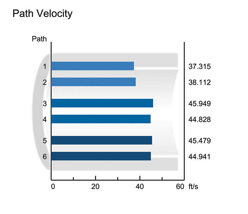
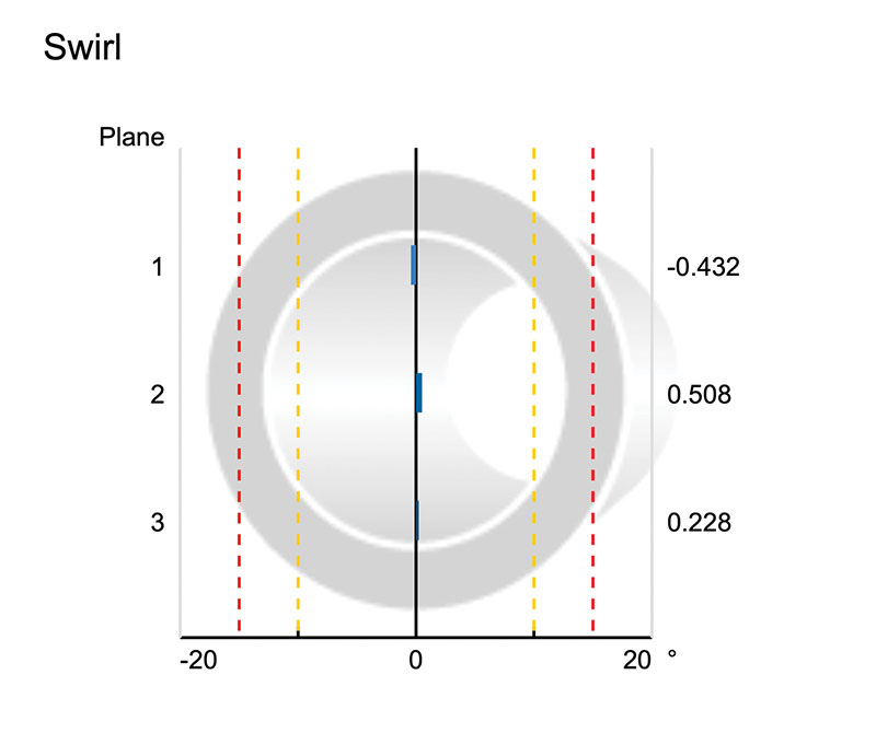
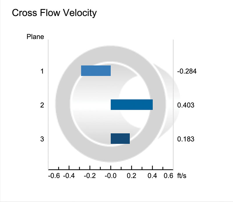
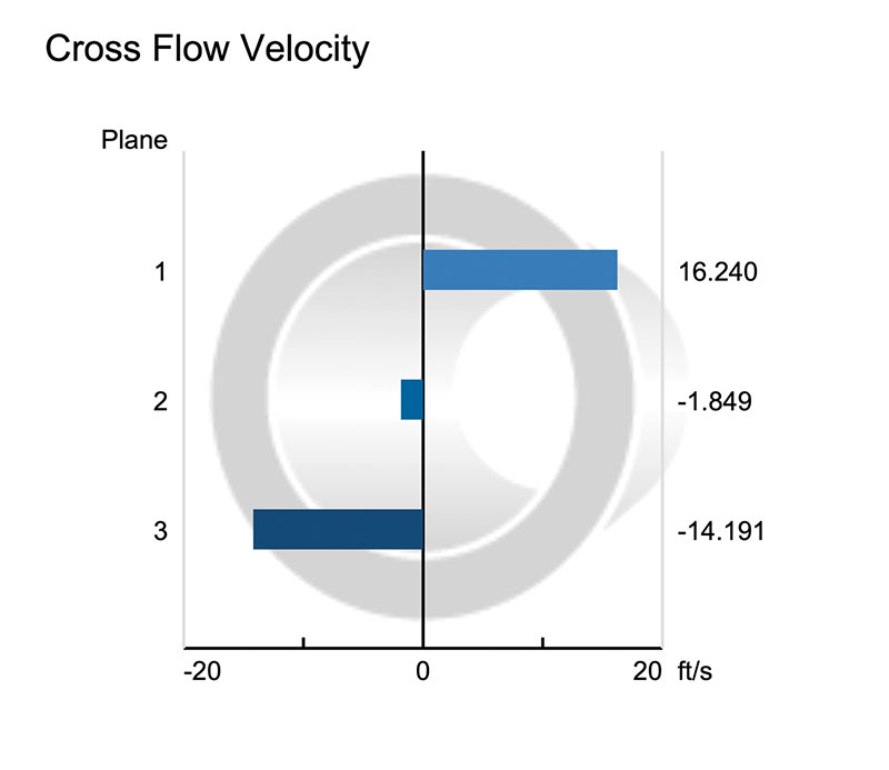
Following are graphs collected during the RT DBOOP FC HMP test, using RMGView software, for three of the most important meter velocity and swirl diagnostics. These graphs were collected during testing at 40 feet per second (fps) and represent diagnostic information for Individual path velocity (Figure 1), swirl by plane (Figure 2) and cross flow velocity by plane (Figure 3).
There are several important diagnostic details shown in these three graphs. First, Figure 1 shows some asymmetry is still present from top to bottom, but the individual path velocities for each plane are very close. This is further supported by Figure 3, which shows extremely little cross flow velocity by plane.
The bar graphs make it look significant because of the graph’s “auto-ranging” feature. However, upon further inspection, it is evident that the amount of cross flow velocity is negligible. Figure 2 shows virtually no swirl for each of the three planes. This data demonstrates just how good the CPA 55E swirl reduction capabilities are.

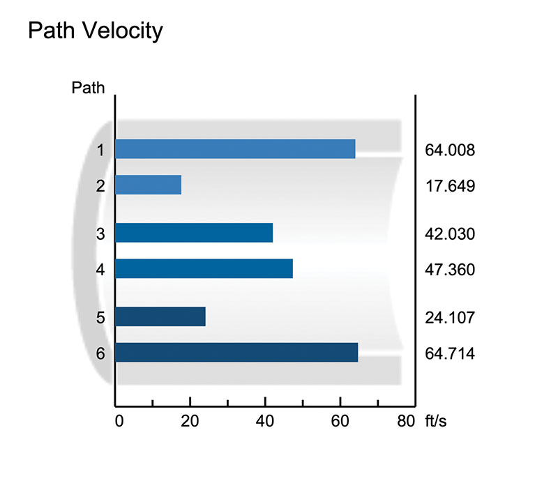
The following diagnostic graphs were obtained from the same upstream piping configuration (RT DBOOP HMP) at 40 fps – but without the CPA 55E. Essentially, this means there were six nominal diameters (ND) upstream of the meter.
Figure 4 shows a tremendous difference in path velocities by plane, especially Paths 1 vs. 2 and Paths 5 vs. 6 where the level of swirl is very high. By comparing the Figure 4 profile with that of Figure 1, a significant difference is apparent. Figure 6 shows the excessive level of cross flow velocity by plane, in particularly Planes 1 and 3.
The cross-flow velocities in Figure 3 were well under 0.5 fps, whereas the values (Figure 6) show velocities in excess of 14 fps. When comparing Figure 5 with Figure 2, it is clear there is a tremendous amount of residual swirl angle by plane that was not present with the CPA 55E.
In Figure 5, both Planes 1 and 3 have active warning and alarm limits. The swirl alarm limit has been exceeded so the meter is now reporting this graph in red as opposed to the blue (Figure 2).
Summary
Today’s gas ultrasonic meter can handle a significant amount of flow profile distortions and still remain within the uncertainty guidelines of the various industry documents. This has been demonstrated by many published papers over the past several years.
However, proving the USM is still accurate once installed in the field, and that it continues to remain accurate over time, is just as important as the initial flow calibration.
The reason clients collect diagnostic log files at the time of flow calibration is to use them to help validate that the meter’s accuracy has not changed significantly once installed in the field.
If a meter is installed without a flow conditioner, flow profile information, as shown in Figures 4 through 6, are nowhere representative of those shown in Figures 1 through 3. Therefore, it would be very difficult to validate that this meter’s accuracy has not been affected by comparing the meter’s diagnostics with and without the CPA 55E.
References
1 AGA Report No. 9, Measurement of Gas by Multipath Ultrasonic Meters, Third Edition, July 2017, American Gas Association, Washington, D.C.
2 Measurement Canada PS-G-06, Provisional specifications for the approval, verification, reverification, installation and use of ultrasonic meters, Revision 4, dated 2017-11-15.
3 ISO 17089-1:2019, Measurement of fluid flow in closed conduits – Ultrasonic meter for gas, August 2019, Second Edition, Geneva, Switzerland.
4 OIML R 137-1 & 2, Edition 2012(E), Including Amendment 2014, International Organization of Legal Metrology.
5 Tech Note 3: Shorter Upstream USM/CPA Piping Lengths Significantly Reduces Cost, John Lansing, November 2020.

Comments