
September 2023, Vol. 250, No. 9
Features
Non-Contact, Drone-Based Technology for Movement Assessment
By Kella Bennani, H., Miaohang, H., Laichoubi, M., Stasse, F., Hart, J.D. and Fathi, A., Enbridge
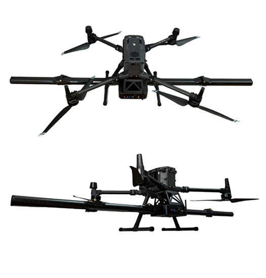
(P&GJ) — Based on its R&D experience, Skipper NDT decided in 2019 to address pipeline geolocation and strain assessment using UAS. This effort has provided a 2.2-kg and a 160-cm wide embedded system that can be easily mounted on any UAS (Figure 1). The main components of the system are:
- Four three-components fluxgate magnetometers
- Real-time Global Navigation Satellite System GNSS receiver with a centimetric-level accuracy
- Tactical grade inertial measurement unit (IMU)
- Telemetric sensors measuring the distance between the magnetometers and the ground (or canopy)
- Proprietary electronic card for data acquisition, digitalization, and synchronization
The system relies on two primary sensors (magnetometers and GNSS) for the acquisition of magnetic data. Of these, the fluxgate magnetometers are particularly crucial, as they can measure the three components of the magnetic field at a sample frequency of 1000 Hz with a mass of 112 g per sensor.
In comparison to scalar magnetometers, fluxgate magnetometers possess sensors that are overall lighter and more resilient, with a sampling frequency that is ten to a hundred times higher, making them more suited to the constraints of UAS. One notable advantage of fluxgate sensors is that they can capture the 3-D components of the magnetic field, making it possible to compensate for the magnetic effect of the embedded equipment and UAS. As a result, the system can be adapted to different vectors without the need for custom characterization.
However, it is important to note that these fluxgate magnetometers are not absolute instruments and may contain errors related to offset, sensitivity, and angle (non-orthogonality), which is compensated for through a proprietary calibration protocol.
Within the scope of our work, it is essential for GNSS hardware to satisfy stringent requirements with respect to both accuracy and weight. Although lightweight GNSS hardware is commonplace in UAS applications, we opted to use a 606-g receiver and antenna system that offers greater technical capabilities.
Moreover, the system is composed of various components that primarily serve a corrective function. Due to the unique demands imposed by airborne systems as compared to ground-based systems, these corrections are essential. To mitigate any heading misalignments with the route, IMU is utilized to perform level control, which corrects the navigation system.
The remote sensors, which incorporate both ultrasonic and Lidar measurements, are used to calculate the distance from the magnetometers to the ground or canopy, enabling the system to precisely infer the depth of the pipeline below the ground surface.
3-D Localization
Skipper NDT has developed an automatic multi-step procedure to derive position profiles of buried pipelines. The first step involves an automatic drone-based inspection that includes boundary demarcation of the inspected area and definition of the drone’s trajectory (Figure 2).
This step enables the collection of data from hard-to-reach or hazardous areas and ensures that the inspection is carried out efficiently and safely. The second step involves data post-processing and exploration, which includes data calibration to reduce noise, and terminates with magnetic map generation (Figure 2).
This step ensures that the collected data is accurate and reliable, and the magnetic map provides a comprehensive overview of the pipeline’s environment. The third point involves magnetic inversion to derive the [Equation] position and depth of cover of the pipeline.
The typical data spacing is 0.5m since it is not necessary for most operators to have a higher definition of their pipeline trajectory for positioning purposes. This data spacing can be reduced to 0.05 m without interpolation. For this case study, the data spacing is equal to 0.06 m to match IMU data spacing. This provides clients with the precise location of the pipeline.
The pre-inspection report is made available on an online platform, allowing for easy and secure access to the pipeline’s position profiles. Figure 2 illustrates a simple localization exercise carried out in coordination with GRTGaz on a buried pipeline.
The data goes through several processing steps: First, the magnetic map is determined. An optimization problem is then solved to find XYZ values. Once XYZ values are obtained, the Ramer-Douglas-Peucker algorithm is applied to separate the result to a set of polylines.
Then a linear regression filter is applied to a typical window length along each section of polylines. For points with an intercept greater than an acceptable value, they are replaced by their projection onto the linear regression line. For other points, we keep their coordinates. Further details regarding the inversion algorithms and validation studies can be found in the references provided [2] and [3].
This article specifically focuses on using the pipeline location data to calculate bending strain profiles and investigate pipeline movements. The following section will outline the general steps followed to develop the horizontal and vertical bending strain profiles using [Equation] position profiles, prior to presenting the case study and validation test.
Bend Strain
Typically, when the pipe material is within its elastic deformation range, the bending strain corresponds to the curvature of the pipeline in a proportional manner. Consequently, by using the position information of the centerline, the curvature of the pipeline can be accurately determined, allowing for the calculation of the pipeline bending strain. The following expression can be used to describe the pipeline bending strain:
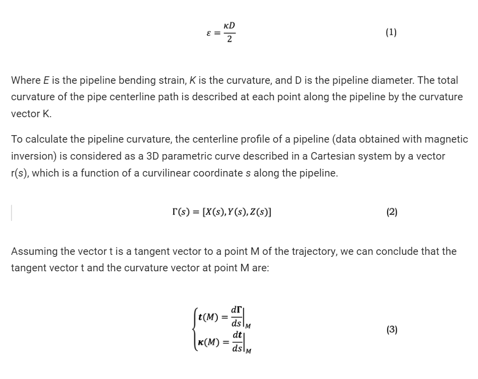
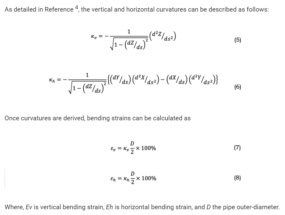
From the above equations, it can be seen that the pipeline bending strain is calculated using the trajectory of centerline path, which can be obtained from the drone-based tool.
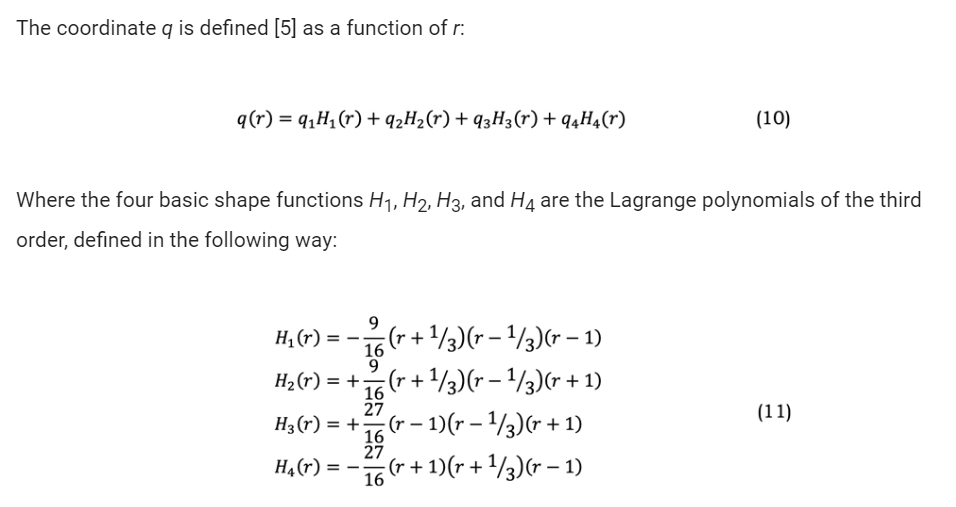
LaGrange Polynomials
One of the key steps in accurately calculating the curvature is to precisely perform differentiation of X, Y, and Z location of the pipeline with respect to the curvilinear path coordinate "s". Interpolation functions provide a powerful tool for achieving this goal as they allow to perform high-order differentiation in a smooth and accurate manner.
By using interpolation functions, we can obtain values of the first and second derivatives at any point along the pipeline. However, it is important to ensure the continuity of the derivatives at the boundaries of each element (an element is defined as a segment between two consecutives discrete XYZ coordinate points).
Several options are available to achieve this goal, such as using polynomial or spline functions, which allow for the smooth joining of adjacent elements while maintaining the continuity of the first and second derivatives.
The surveyed pipe centerline path is defined using discrete XYZ position coordinates at a grid of discrete along-pipe distance values “s.” Typical surveys result in a path distance between coordinates of about 0.1 meter. The surveyed section of the pipeline is partitioned into discrete elements of constant in-situ curvature (Figure 3) in between the discrete position coordinates. The model approximates each of the X, Y and Z datasets in each element as a cubic polynomial of the curvilinear coordinate "s". To simplify the analytical definition of real elements, an isoparametric element is introduced. Such a reference element may be transformed into any real element by the geometrical transformation (s) described by:
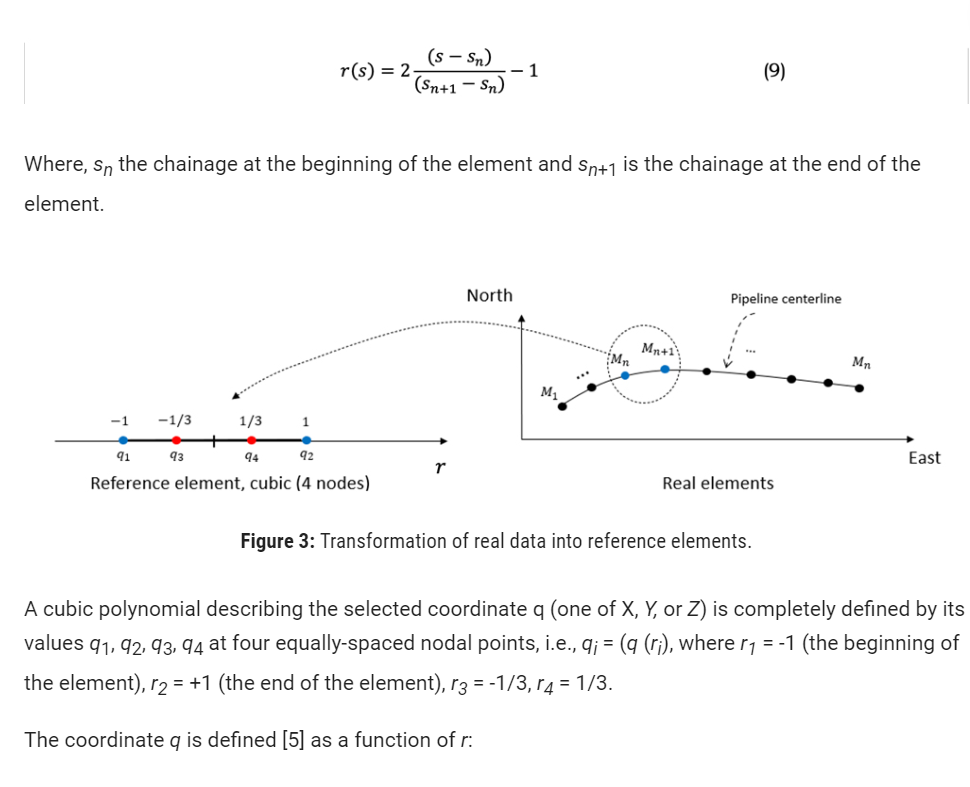
Each element has four degrees of freedom for each coordinate (X, Y, Z). It is assumed that the coordinates are continuous at the element boundaries together with imposed continuity of the first/second derivatives (tangent/curvature vectors) at the element boundaries.
As a preliminary test of our ability to detect bends due to permanent ground movements, we collaborated with Enbridge and selected a site that contained a small cold bend, which could approximately simulate certain aspects of the behavior of a pipeline subject to permanent ground displacement.
The following section presents a case study and a comparison of the results obtained using our drone-based tool against those obtained with an IMU survey tool.
Case Study
Our technology has a primary application of detecting pipeline bending signatures caused by landslides before they pose a significant threat to pipeline integrity.
To achieve this, site selection was conducted in collaboration with a North American pipeline operator, using two primary criteria. The first criterion was that the site should contain a small cold bend that can simulate aspects of the curvature changes resulting from permanent ground displacement.
The second criterion focused on selecting sites for which IMU survey data was available for comparison. Ultimately, a 500-meter length, 24-inch pipeline (Figure 4) was selected that had a 2.5° horizontal cold bend. Figure 4 describes the inspected area where, red polygon corresponds to limits of the inspection area. White lines correspond to the trajectory followed by the drone during this mission.
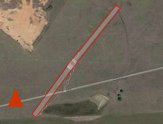
In this inspection, drone-based technology was used to collect data on the pipeline’s magnetic map. The average magnetic map dimension was 590-by-5 meters by 7 profiles. The drone flew at an average height of 2 meters, with an average flying speed of 6,5-km per hour. The acquisition time for the inspection was 45 minutes.
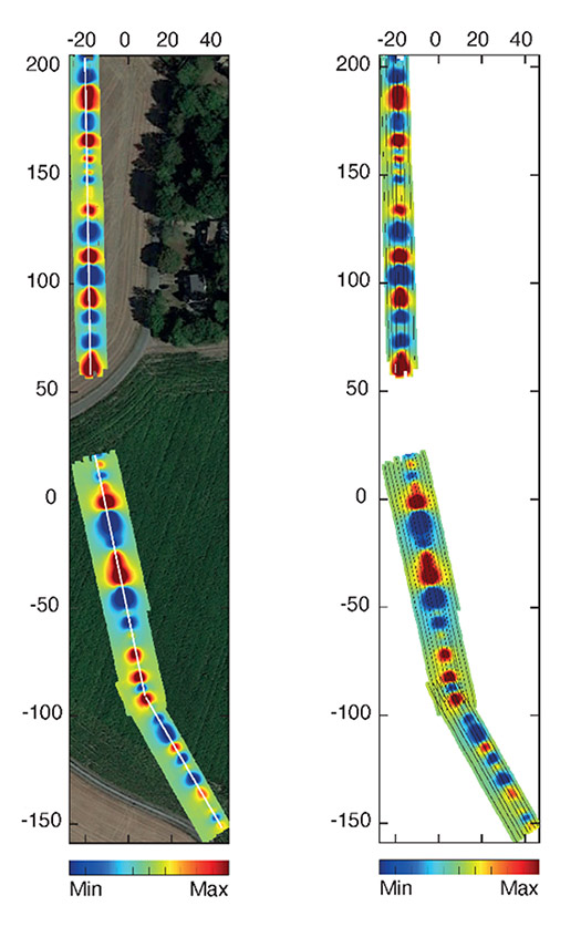
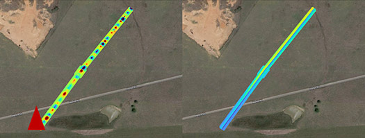
Once the field data acquisition was completed, the collected magnetic signals were calibrated and filtered to remove any noise or interference. Then, the data need to be interpolated to fill in any gaps or missing data points. Finally, the processed data can be used to create magnetic maps to be inverted (Figure 5) for low- and high-frequency. Based on the magnetic map (low frequency) illustrated in Figure 5, two conclusions can be drawn: First, there is a noticeable intensification of the magnetic spots in the area corresponding to cold bends in the pipeline.
These bends generally cause the magnetic field in the area to be amplified, leading to a more pronounced magnetic signature on the map. Secondly, an unusual magnetic spot is localized near the end of the surveyed section of the pipeline, which corresponds to a sudden change in curvature. This location corresponds to an intentional cold overbend-sagbend sequence.
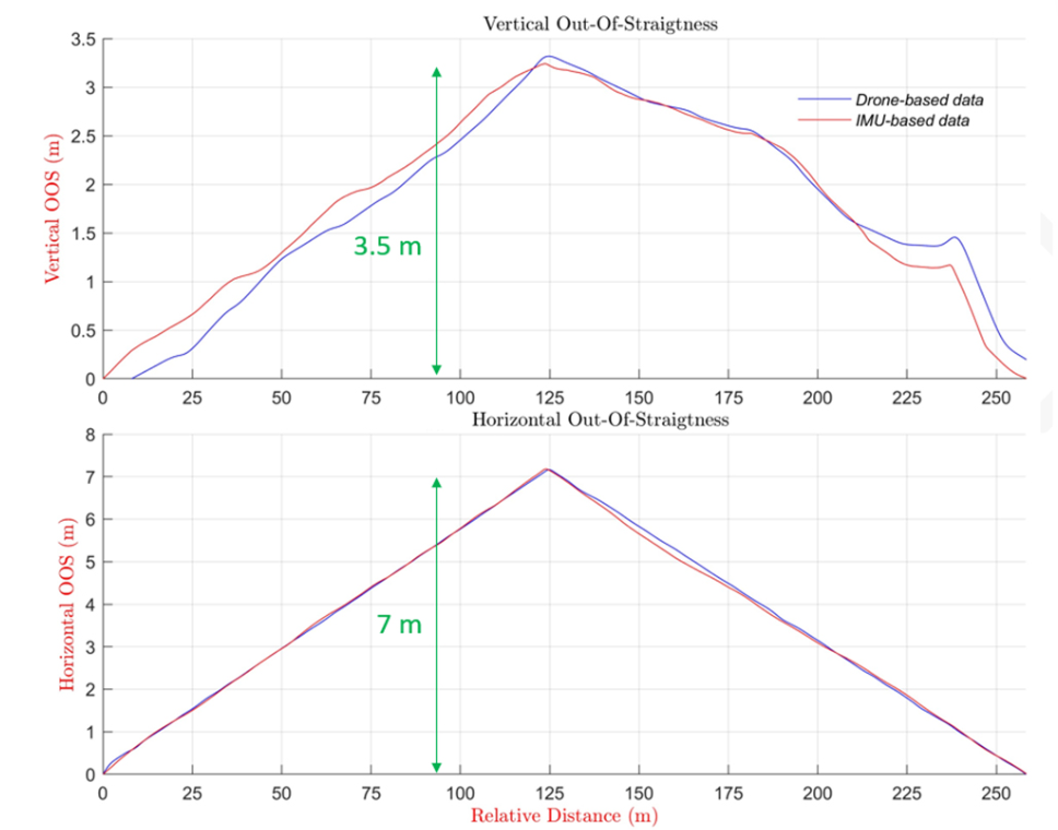
To visualize subtle changes in the centerline of the pipeline, we utilize out-of-straightness (OOS) profiles, which are defined as the horizontal and vertical deviation from a straight line connecting the start and end points. This metric is particularly useful in analyzing small pipeline deflections and can be a reliable indicator of potential ground movement signatures.
To provide a comparative analysis of the OOS profiles generated by our drone-based tool, we have also included IMU data provided by the operator and obtained through a previous in-line inspection.
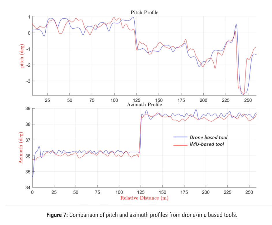
Before developing bending strain profiles, it is necessary to evaluate the orientation profile deviation along the pipeline. One way to do this is by analyzing the azimuth/pitch orientation profiles. The azimuth/pitch profiles capture the directional trend of the pipeline, which can be readily compared to those provided by IMU survey data.
There is a reasonably good agreement between the two datasets (Figure 6), indicating that our drone-based technology was able to accurately capture the orientation change trends. Furthermore, the comparison revealed a 2.5° change in the pipeline orientation, which was well-captured by our technology.
Once the location data is at hand, we develop the vertical/horizontal out-of-straightness using procedures developed [6].
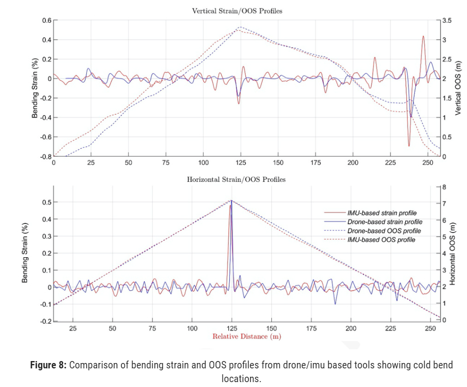
In Figure 8, the blue curve obtained from the drone-based approach was compared with the results (red curve) of an inline inspection to evaluate the changes in orientation and bending strain. The developed bending strain profiles obtained with both technologies are illustrated.
With respect to the horizontal view (bottom), the cold bend located at 125 m is distinctly identified and captured. Elsewhere, in the straight parts, the noise has been minimized using a modified linear regression filter. Concerning the vertical out-of-straightness (top), there is a sudden curvature change near the end of the surveyed section of the pipeline which corresponds to a strain peak that is well-identified using both technologies. It is worth noting that we have missed some peaks at both 210 m and 235 m.
The primary reason for this inaccuracy is the less precise GNSS positioning in the Z (vertical) axis, which could be improved on our part through the implementation of Post Processed Kinematic (PPK) corrections using a permanent base to enhance positioning [7]. Finally, the comparison revealed a reasonably satisfactory level of agreement between the two sets of data, thereby instilling confidence in the accuracy of our approach.
The preliminary test, conducted in coordination with Enbridge, demonstrated the efficiency of our technology in performing bending strain analysis, especially in the horizontal direction. This result is a promising indication of the potential of our technology in the pipeline industry. However, it is important to note that this is a single instance and, therefore, further data and testing are necessary to provide a more comprehensive assessment of our technology’s capabilities for bending strain evaluation.
Rigorous testing and evaluation will enable us to quantify our performance metrics and validate the reliability of our approach. However, we must continue to refine and improve our approach through additional testing and evaluation to ensure the accuracy and reliability of our methodology.
Bending Strain
The results presented above indicate that the contactless drone-based magnetic technology enables a preliminary curvature-based analysis to identify potential zones of distress/failure. This can be highly advantageous for operators in several ways:
- Firstly, the use of this technology is rapid, meaning that the process of identifying potential failure zones can be completed quickly. This is especially useful when time is of the essence, and immediate action needs to be taken. This will enable operators to take necessary remedial actions to ensure the safety of pipeline operations and comply with regulations.
- Secondly, the technology can be deployed in difficult-to-reach areas, which may not be easily accessible by conventional inspection methods.
- Finally, one of the major advantages of using a drone-based tool is that it can be designed to operate without the need for human intervention. Reducing the risk of human error and improving personnel safety.
Hence, the multi-step procedure described in Section 2.1 can be complemented with two additional steps (Figure 9) to assess pipeline movements and bending strain profiles for geohazard management purposes.
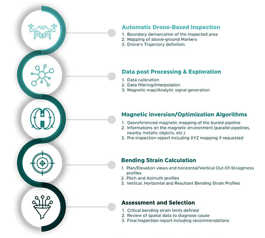
These steps consist of developing vertical and horizontal pipe curvature/bending strain profiles. This provides a more detailed analysis of the pipeline’s condition and helps identify areas of concern.
The second step focuses on the assessment and prioritization of the zones where strain limits are exceeded. This ensures that the client has a comprehensive understanding of the pipeline’s integrity, and any potential issues are identified and addressed promptly.
This five-step process can be declined in various ways to address a broad range of remote services listed (Figure 10). These services can help ensure the safety of buried pipelines, reduce downtime and maintenance costs.
Perspectives
The method presented in this study demonstrates promising results in terms of positioning and out-of-straightness assessment when compared to the “gold standard” (IMU). After applying an adapted filter to the signal, the strain profiles for both horizontal and vertical strains on the Enbridge use case reasonably match the IMU based curves.
Despite the excellent detection performance, the strain values are underestimated, particularly on the vertical axis. Notably, these results were obtained after 40 minutes of cumulative flight time only, and without any interruption to the pipeline flow.
This technology is designed to be a screening tool that provides a rapid response in landslide or other geohazard situations. The signature geometry of real-life landslides is less abrupt in XY and Z than the sharp cold bends considered in this use case [8].
Consequently, the drone-based magnetic inspection results will likely be much better for the end use application. Ideally drone surveys can distinguish between ground movement signatures and intentional bend (cold bends, induction bends, elbows) signatures [9].
In addition to serving as a validation tool, the technology can also be used in between two ILI runs. When IMU deployment is time consuming and logistically challenging our technology can help fill the gap by providing clients with quick and reliable data on the condition of their pipelines with direct overlay comparisons with the most recent previous IMU survey. This enables them to stay up to date with the status of their pipelines, even when a full IMU inspection is not possible.
Finally, to enhance the competitiveness of our technology in the market, it is imperative that we address several key factors in a coordinated effort, ideally in collaboration with a prominent industry leader. Among the measures that ought to be implemented to capitalize on the favorable outcomes achieved:
- Confirm the solid results obtained by comparing our bending strain results at known geohazard sites against recent IMU data. This will enable us to establish the relative accuracy of the strain estimation. Ideally this would be done with 5 to 10 locations in varying conditions to understand how certain variables can affect our accuracy of strain estimation.
- Refine the filtering to find the best parameters if a unique set exists. If not, find a method to adapt the filtering to each case.
- Enhance the vertical strain estimation by improving the vertical positioning. This issue is most certainly due to GNSS capabilities that are typically better in XY positioning and it can be addressed by using GNSS corrections like PPK.
Disclaimer: Any information or data pertaining to Enbridge Employee Services Canada Inc., or its affiliates, contained in this paper was provided to the authors with the express permission of Enbridge Employee Services Canada Inc., or its affiliates. However, this paper is the work and opinion of the authors and is not to be interpreted as Enbridge Employee Services Canada Inc., or its affiliates’, position or procedure regarding matters referred to in this paper. Enbridge Employee Services Canada Inc. and its affiliates and their respective employees, officers, director and agents shall not be liable for any claims for loss, damage or costs, of any kind whatsoever, arising from the errors, inaccuracies or incompleteness of the information and data contained in this paper or for any loss, damage or costs that may arise from the use or interpretation of this paper.
References:
[1] Munshy M, Boulanger D, Ulrich P, Bouiflane M. “Magnetic Mapping for the Detection and Characterization of UXO: Use of Multi-Sensor Fluxgate 3-axis Magnetometers and Methods of Interpretation “. Use full citation.
[2] M. Laichoubi et al, “Automatic 3D-localisation of buried Pipeline and depth of Cover: Magnetic Investigation under Operational Conditions. “ Use full citation.
[3] M. Laichoubi et al, “3D-Localisation and Magnetic Mapping of Buried Pipelines Using unmanned Aerial System. “ Use full citation.
[4] Czyz, J.A. and Adams, J.R., “Computation of Pipeline Bending Strains Based on Geopig Measurements “, Proceedings of the Pipeline Pigging and Integrity Monitoring Conference, Houston TX, February 14-17, 1994.
[5] Rui Li et al., “Development the method of pipeline bending strain measurement based on microelectromechanical systems inertial measurement unit. “ Use full citation.
[6] Hart, J.D., Zulfiqar, N., and McClarty, E., “Recommended Procedures for Evaluation and Synthesis of Pipelines Subject to Multiple IMU Tool Surveys “, IPC2020-9235, Proceedings of the 13th International Pipeline Conference, Calgary, Alberta, Canada, September 28-October 2, 2020.
[7] N. A. Famiglietti, G. Cecere, C. Grasso, A. Memmolo, and A. Vicari, “A test on the potential of a low cost unmanned aerial vehicle rtk/ppk solution for precision positioning, “ Sensors, vol. 21, no. 11, Jun. 2021, doi: 10.3390/s21113882.
[8] A. Fathi, O. Ndubuaku Stantec, C. Edmonton, C. Nader Yoosef-Ghodsi, and M. Hill, “Rapid Strain Demand Estimation of Pipelines Deformed by Lateral Ground Movements, “ 2020.
[9] Hart, J.D., Czyz, J.A. and Zulfiqar, N., “Review of Pipeline Inertial Surveying for Ground Movement-Induced Deformations “, AIM-PIMG2019-1009, Proceedings of the Conference on Asset Integrity Management-Pipeline Integrity Management Under Geohazard Conditions, Houston, TX, USA, March 25-28, 2019.

Comments