November 2024, Vol. 251, No. 11
Features
Comprehensive Review and Comparative Study of Risk Models
By Eduardo Munoz, Principal Consultant, Dynamic Risk
(Editor’s note: This is the second of a two-part article. Part 1 appeared in the October edition of P&GJ.)
Risk models are prominent pipeline integrity management (PIM) tools used to make data-driven decisions. As computing power has increased and data acquisition methods have proliferated, risk models have become more complex.
Moreover, the transition to quantitative risk assessment (QRA) techniques and the heightened intricacy of the corresponding risk models requires a greater amount of specific high-quality information to be provided as inputs for the risk models, including metadata generated during their production.
In Part 2, we turn our attention to case studies for further illustration.
Most qualitative risk assessment (QRA) models calculate a probability of exceedance (POE), or probability of failure (POF) based on the In-Line Inspection (ILI) tool capabilities coupled with fitness-for-service (FFS) calculators. For example, a simple probabilistic corrosion model would perform a Monte-Carlo analysis to assess the limit state of the wall loss indications reported by the latest ILI run.
FFS calculators, such as Modified ASME B31G and Modified LnSec, have been validated, and their degree of conservatism and application range has been reported. However, a SA is not usually part of the validation process.
Yet, a sense of the parameters affecting the estimated burst pressure has been developed from the constant use of the FFS calculators; safety factors affecting the flaw dimensions are commonly introduced to compensate for the inaccuracy inspection technique, and flaw depth is considered to have more impact on the outcome than the other two flaw dimensions.
The ASME Modified B31G Remaining Strength of Corroded Pipeline methodology (Mod B31G) is commonly used for the burst pressure calculations (i.e. the limit state) for corrosion features.
Two different domains were considered for the SA of the burst pressure calculator: (1) an extended domain that covers as many combinations as possible of pipe dimensions, material properties and flaw sizes, and (2) selected cases with representative size and material property variations within a single pipe, and flaw measuring errors (i.e., sizing accuracy) representative of the current inspection methods.
The intervals for the pipe dimensions (D and t) were selected to represent the inventory installed with most operators in North America. An additional condition of 4t < D was introduced. There are some limitations to the linear distributions: outside diameter and wall thickness of installed vintage pipe are generally limited to the combinations specified in an earlier version of API 5L.
In addition, some combinations would not be realistic from an engineering perspective, such as thin-walled pipe with a large diameter. Still running such a general case is essential to assess the applicability of the model. The parametrization used for the first scenario is presented in the following Table:
Table 3: Proposed parametrization for Mod B31G scenario 1
|
Parameter |
Variable |
Units |
Distribution |
Min Value |
Max Value |
|
X1 |
D |
in |
Uniform |
2 |
60 |
|
X2 |
l |
in |
Uniform |
1 |
100 |
|
X3 |
t |
in |
Uniform |
0.1 |
0.5 |
|
X4 |
d |
in |
Uniform |
0.05*t |
0.8*t |
|
X5 |
YS |
psi |
Uniform |
20,000 |
85,000 |
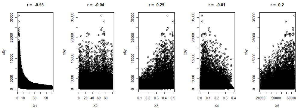
(Figure 1) presents an array of scatter plots correlating five distinct risk variables (X1 through X5) with the model output (Y). Each plot is annotated with a Pearson correlation coefficient (r), indicative of the strength and direction of the linear relationship between the corresponding risk variable and the output.
The values of the Pearson correlation coefficient range from -1 to +1, where +1 implies a perfect positive linear correlation, 0 indicates no linear correlation, and -1 represents a perfect negative linear correlation.
For X1 (the outside diameter), we observe a strong negative linear correlation (r = -0.55), suggesting that as X1 increases, Y (the burst pressure) tends to decrease.
In contrast, X2 (flaw length) exhibits an r value of -0.04, which points to a negligible linear relationship with Y. Similarly, X4 (flaw depth) shows an r value of -0.01, further indicating a lack of any significant linear correlation with the output. X3 (wall thickness) and X5 (yield strength), with r values of 0.25 and 0.2, respectively, demonstrate weak positive linear relationships, indicating that higher values of these variables are associated with higher output values to a small degree.
These scatter plots are instrumental in identifying which risk variables have a more pronounced linear influence on the output, thus guiding risk management strategies.
Variables with higher absolute values of the Pearson correlation coefficient, such as X1 (outside diameter), are likely to be prioritized for control or mitigation due to their stronger linear association with the output.

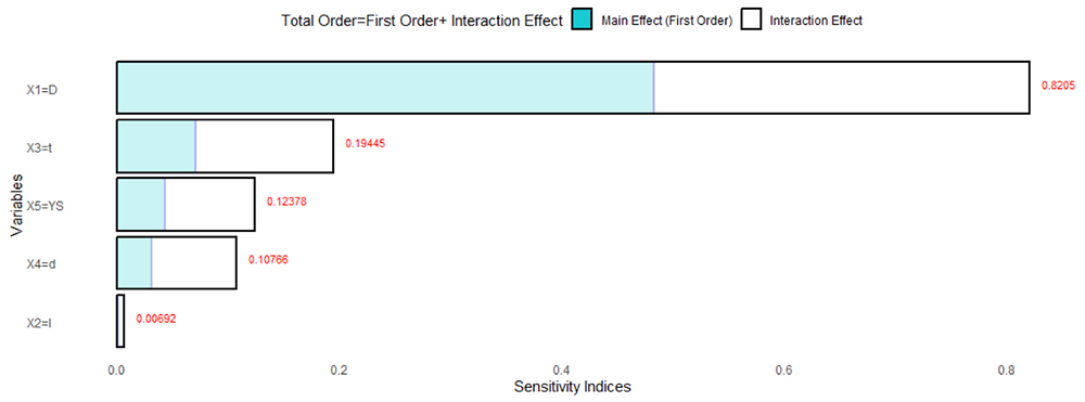
The tornado chart (Figure 2) shows the sensitivity indices for the set of input variables, namely X1 through X5, in relation to the output of the Mod B31G model (burst pressure). Each horizontal bar represents the extent of influence that each variable exerts, with the main effects delineated in turquoise and the interaction effects in white.
From the chart, it is discernible that the outside diameter (X1) stands out with the highest total order sensitivity index, demonstrating the most significant combined effect on the model’s output.
This is evidenced by the turquoise segment of the bar corresponding to X1, which extends considerably further than those of the other variables, coupled with an interaction effect denoted by the white segment, culminating in a total index of approximately 0.8205.
In contrast, flaw length (X2) exhibits the least influence with a negligible main effect and an inconsequential interaction effect, leading to a minimal total sensitivity index close to 0.00692. The other variables, pipe wall thickness (X3) and flaw depth (X4), depict moderate main effects and very minor interaction effects, with total sensitivity indices of approximately 0.19445 and 0.12378, respectively.
Meanwhile, Yield Strength (X5) presents a slight main effect and a total index of about 0.10766. In this general case, pipe dimensions are the factors with more impact on the outcome (i.e., higher sensitivity factors), followed by the material properties (YS). On the contrary, the flaw dimensions are the factors with the least impact upon Mod B31G, in the general case.

Three additional scenarios corresponding to actual flaw assessments were considered. The pipe dimensions consider the local variations along a single pipe. The yield strength distribution corresponds to the variations reported for API 5L Grade B and flaw size corresponds to common ILI tool accuracy: the flaw depth accuracy was assumed to be within 10% the size for 99.7% of indications, while the length accuracy was assumed to be within 20% the size for 99.7% of indications.
Scenario A corresponds an API 5L Grade B, 3-in pipe with a wall loss of 50% of the pipe wall and a flaw length of 25 in. Scenario B is an API 5L Grade B, 12.5-in pipe with a wall loss of 50% of the pipe wall and a flaw only 2 in long. Scenario C corresponds to an API 5L Grade B, 25-in pipe and a 50-in long flaw with a depth of 50% the pipe wall thickness. Table 4 presents the parametrization used for scenarios A, B and C.
Table 4: Proposed parametrization for Mod B31G (scenarios A to C)
|
|
|
|
|
Scenario A |
Scenario B |
Scenario C |
|||
|
Parameter |
Variable |
Units |
Distribution |
Mean |
STD |
Mean |
STD |
Mean |
STD |
|
X1 |
D |
In |
Normal |
3 |
0.0018 |
12.5 |
0.0075 |
25 |
0.0018 |
|
X2 |
l |
In |
Normal |
25 |
0.75 |
2 |
0.06 |
50 |
1.5 |
|
X3 |
t |
In |
Normal |
0.15554 |
0.00154 |
0.22119 |
0.00219 |
0.37875 |
0.00375 |
|
X4 |
d |
In |
Normal |
0.077 |
0.00513 |
0.1095 |
0.0073 |
0.1875 |
0.0125 |
|
X5 |
YS |
Psi |
Normal |
38,500 |
1,225 |
38,500 |
1,225 |
38,500 |
1,225 |
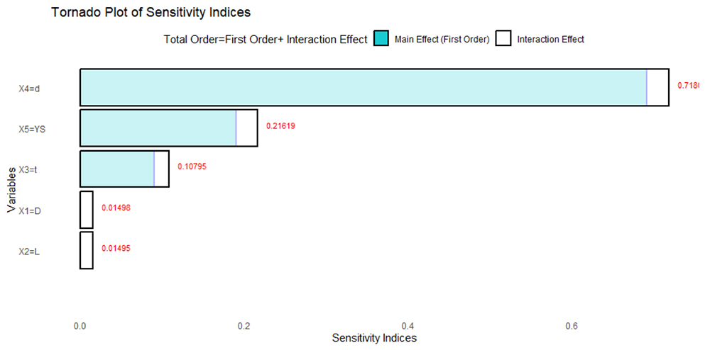
The tornado chart (Figure 3) shows the sensitivity indices for Scenario A. The flaw depth (X4) has the highest total order sensitivity index. Yield Strength (X5) comes second, with more influence on the outcome than the pipe dimensions. Pipe wall thickness (X3) depict a moderate effect with total sensitivity index of approximately 0.19445.
Outside diameter (X1) and flaw length (X2) have the least impact on the model outcome with a total sensitivity index of approximately 0.015. It can be observed that the interaction effect corresponds to less than 10% of the total sensitivity index for the top three factors.

Table 5 presents the sensitivity factors for scenarios A, B and C. It should be noted that the flaw length has the least impact on the outcome in Scenarios A and C but has the highest sensitivity index for scenario B.
Scenario B corresponds to a short wall loss indication in the axial direction, while keeping the same size accuracy as the other two scenarios, which might not be realistic, since some ILI tools have a threshold for flaw detection to a few different accuracies, depending on the flaw size.
However, the mentioned effect of the flaw length parameter in Mod B31G illustrates the need to run SA on multiple cases representative of the operator assets. That is, the general case shown in Scenario 1 does not suffice and the sensitivity cases used for the analysis of one system should be reviewed before using with another system, to make sure they are representative.
Table 5: Sensitivity factors for Mod B31G (scenarios A to C)
|
|
|
Sensitivity Analysis |
||
|
Parameter |
Variable |
Scenario A |
Scenario B |
Scenario C |
|
X1 |
D |
0.015 |
0.007 |
0.015 |
|
X2 |
l |
0.015 |
0.724 |
0.015 |
|
X3 |
t |
0.108 |
0.05 |
0.079 |
|
X4 |
d |
0.718 |
0.093 |
0.683 |
|
X5 |
YS |
0.216 |
0.19 |
0.272 |
FFS subject matter experts have stressed the importance of flaw depth on the outcome of the burst pressure calculation of corroded pipe; flaw depth is indeed the parameter with most influence on the burst pressure calculation.
However, in some cases, the values and accuracies of the other factors might Hence, the importance of performing the SA for each risk model — with cases representative of the system and the inspection tools used — coupled with the results with the data uncertainty assessment. YS consistently comes in the top three influential factors. The original Mod B31G model uses SMYS rather than YS.
The SA presented shows that original simplification has impact on the calculated burst pressure, and that the calculation would benefit from the use of representative mechanical properties rather than minimum specified values.
Compliant Risk Model
The SA of a risk model was performed. The model considers all threats specified in ASME B31.8S Section 2 and the Safety, Environmental and Production Loss for Consequence of Failure (CoF). The final Likelihood of Failure (LoF) is calculated by simple aggregation of the LoF of individual threats. Table 6 shows a summary of the models used for each threat.
Table 6: Basis of the assessed risk model
|
Threat |
Model Basis |
|
External Corrosion |
Mod B31G |
|
Internal Corrosion |
Mod B31G |
|
Stress Corrosion Cracking |
Mod Ln Sec for Axial Cracking |
|
Manufacturing - Defective Pipe Seam |
Mod Ln Sec for Axial Cracking |
|
Manufacturing - Defective Pipe |
Mod Ln Sec for Axial Cracking |
|
Defective Girth Weld |
Simple Limit State Thresholds |
|
Defective Fabrication Weld |
Susceptibility Model |
|
Wrinkle Bend or Buckle |
Susceptibility Model |
|
Equipment Failure |
API 581 |
|
Third Party Damage |
Impact model by Chen and Nessim coupled with probability of failure given a hit model by Fuglem et al. |
|
Previously Damaged Pipe |
EPRG Mechanical Damage Fatigue Model |
|
Incorrect Operational Procedure |
CEPA IF Self-Assessment Questionnaires |
|
Weather Related and Outside Force |
Geohazard and hydro hazard mapping coupled with lateral strain measurements |
Table 7 shows the five factors that have the highest effect on the outcome of the risk model. Outside diameter stands out as the predominant parameter, exerting a significant impact on both LoF and CoF.
Yield Strength affects the resistance of the pipe and affects the outcome of the LoF in the majority of the individual threat models. Flaw dimensions (corrosion/crack/gouge depth) were expected to have a significant impact on LoF; however, they rank behind the dimensions of the pipe and the properties of its material in terms of significance.
Table 7: Top 5 influential factors on the risk model
|
Rank |
Symbol |
Parameter |
|
1 |
D |
Outside Diameter |
|
2 |
YS |
Yield Strength |
|
3 |
d |
Wall loss/Crack Flaw Depth |
|
4 |
dg |
Gouge Depth |
|
5 |
MAOP |
Maximum Allowable Operating Pressure |
The above results were integrated to develop data quality flags that influenced the calculated risk. Those quality flags controlled if the pipe dimensions and mechanical properties had Traceable, Verifiable and Complete (TVC) files and if the maximum allowable operating pressure (MAOP) had been reconfirmed.
The risk model was modified to adjust the outcome when data pipe dimensions or mechanical properties were deemed uncertain. Flaw dimensions were considered in the probabilistic LoF analysis that incorporates the measuring tool error and did not require further adjustment in the risk model.
Conclusions
This comprehensive review and comparative study have underscored the critical role of SA in risk assessment for oil and gas pipelines.
Through the meticulous examination of various SA techniques, ranging from variance-based methods to derivative-based and local approaches, the study has highlighted the unique strengths and limitations of each method in the context of pipeline risk management.
A comparative analysis revealed that while some methods like eFAST method provide a broad and detailed sensitivity spectrum, others, such as the Morris Method, offer a more computationally efficient — albeit less accurate and detailed — perspective.
This diversity in SA techniques underscores the necessity of selecting an approach that aligns with specific project requirements, taking into consideration factors such as model complexity, data availability and computational resources.
The practical case of a SA for ASME Mod B31G model for corroded pipe was presented. Scenarios with an extended domain corresponding to the inventory installed and selected cases for representative corrosion features were reviewed. The factors impacting the outcome of the model are dependent on the parametrization.
Hence, a comprehensive SA requires the careful definition of such scenarios to represent the application domain of the risk model.
A ranking of the factors impacting the outcome of a risk model, compliant with ASME/ANSI B38.1S, was presented: pipe dimensions (outside diameter) and mechanical properties (yield strength) are more influential than flaw dimensions (corrosion/crack/gouge depth). The insights, provided by the SA of the risk model, were integrated into the model to compensate for data uncertainty.
Editor’s Note: This paper was originally presented at Clarion’s Pipeline Pigging Integrity Management Conference 2024.
References
[1] Pipeline and Hazardous Materials Safety Administration (PHMSA), RIN 2137–AF39 Pipeline Safety: Safety of Gas Transmission Pipelines: Repair Criteria, Integrity Management Improvements, Cathodic Protection, Management of Change, and Other Related Amendments, 2022.
https://www.federalregister.gov/documents/2022/08/24/2022-17031/pipeline-safety-safety-of-gas-transmission-pipelines-repair-criteria-integrity-management (accessed December 2, 2023).
[2] M. Ionescu-Bujor, D.G. Cacuci, A Comparative Review of Sensitivity and Uncertainty Analysis of Large-Scale Systems—I: Deterministic Methods, Nuclear Science and Engineering 147 (2004) 189–203. https://doi.org/10.13182/NSE03-105CR.
[3] A. Ahmadi-Javid, S.H. Fateminia, H.G. Gemünden, A Method for Risk Response Planning in Project Portfolio Management, Project Management Journal 51 (2020) 77–95. https://doi.org/10.1177/8756972819866577.
[4] S.H. Fateminia, N.G. Seresht, A.R. Fayek, Evaluating Risk Response Strategies on Construction Projects Using a Fuzzy Rule-Based System, in: Proceedings of the 36th International Symposium on Automation and Robotics in Construction, ISARC 2019, 2019: pp. 282–288. https://doi.org/10.22260/ISARC2019/0038.
[5] S.H. Fateminia, P.H.D. Nguyen, A.R. Fayek, An Adaptive Hybrid Model for Determining Subjective Causal Relationships in Fuzzy System Dynamics Models for Analyzing Construction Risks, CivilEng 2 (2021) 747–764.
[6] S.H. Fateminia, A.R. Fayek, Hybrid fuzzy arithmetic-based model for determining contingency reserve, Autom Constr 151 (2023) 104858. https://doi.org/https://doi.org/10.1016/j.autcon.2023.104858.
[7] S.H. ‘Fateminia, Determining and Managing Contingency Reserve throughout the Lifecycle of Construction Projects, PhD Thesis, University of Alberta, 2023.
[8] A. Saltelli, K. Aleksankina, W. Becker, P. Fennell, F. Ferretti, N. Holst, S. Li, Q. Wu, Why so many published sensitivity analyses are false: A systematic review of sensitivity analysis practices, Environmental Modelling & Software 114 (2019) 29–39. https://doi.org/https://doi.org/10.1016/j.envsoft.2019.01.012.
[9] A. Saltelli, R. Marco, A. Terry, C. Francesca, C. Jessica, G. Debora, S. Michaela, T. Stefano, Global Sensitivity Analysis: The Primer, in 2008. https://api.semanticscholar.org/CorpusID:115957810.
[10] R. Ghanem, D. Higdon, H. Owhadi, Handbook of uncertainty quantification, Springer, 2017.
[11] S.H. Fateminia, V. Sumati, A.R. Fayek, An Interval Type-2 Fuzzy Risk Analysis Model (IT2FRAM) for Determining Construction Project Contingency Reserve, Algorithms 13 (2020) 163. https://doi.org/10.3390/a13070163.
[12] S.H. Fateminia, N.B. Siraj, A.R. Fayek, A. Johnston, Determining Project Contingency Reserve Using a Fuzzy Arithmetic-Based Risk Analysis Method, in: Proceedings of the 53rd Hawaii International Conference on System Sciences, Hawaii International Conference on System Sciences, 2020. https://doi.org/10.24251/hicss.2020.214.
[13] S. Razavi, A. Jakeman, A. Saltelli, C. Prieur, B. Iooss, E. Borgonovo, E. Plischke, S. Lo Piano, T. Iwanaga, W. Becker, The future of sensitivity analysis: An essential discipline for systems modeling and policy support, Environmental Modelling & Software 137 (2021) 104954.
[14] E. Borgonovo, G.E. Apostolakis, S. Tarantola, A. Saltelli, Comparison of global sensitivity analysis techniques and importance measures in PSA, Reliab Eng Syst Saf 79 (2003) 175–185. https://doi.org/https://doi.org/10.1016/S0951-8320(02)00228-4.
[15] E. Borgonovo, E. Plischke, Sensitivity analysis: A review of recent advances, Eur J Oper Res 248 (2016) 869–887. https://doi.org/https://doi.org/10.1016/j.ejor.2015.06.032.
[16] D.G. Cacuci, M. Ionescu-Bujor, A Comparative Review of Sensitivity and Uncertainty Analysis of Large-Scale Systems—II: Statistical Methods, Nuclear Science and Engineering 147 (2004) 204–217. https://doi.org/10.13182/04-54CR.
[17] A. Saltelli, R. Marco, A. Terry, C. Francesca, C. Jessica, G. Debora, S. Michaela, T. Stefano, Global Sensitivity Analysis: The Primer, in 2008. https://api.semanticscholar.org/CorpusID:115957810.
[18] C. Xu, G.Z. Gertner, Uncertainty and sensitivity analysis for models with correlated parameters, Reliab Eng Syst Saf 93 (2008) 1563–1573. https://doi.org/https://doi.org/10.1016/j.ress.2007.06.003.
[19] E. Borgonovo, Sensitivity Analysis, in: Tutorials in Operations Research: Advancing the Frontiers of OR/MS: From Methodologies to Applications, INFORMS, 2023: pp. 52–81. https://doi.org/doi:10.1287/educ.2023.0259.
[20] I.M. Sobol’, S. Kucherenko, Derivative based global sensitivity measures and their link with global sensitivity indices, Math Comput Simul 79 (2009) 3009–3017. https://doi.org/https://doi.org/10.1016/j.matcom.2009.01.023.
[21] I.M. Sobol′, Global sensitivity indices for nonlinear mathematical models and their Monte Carlo estimates, Math Comput Simul 55 (2001) 271–280. https://doi.org/https://doi.org/10.1016/S0378-4754(00)00270-6.
[22] R.I. Cukier, C.M. Fortuin, K.E. Shuler, A.G. Petschek, J.H. Schaibly, Study of the sensitivity of coupled reaction systems to uncertainties in rate coefficients. I Theory, J Chem Phys 59 (1973) 3873–3878.
[23] E. Plischke, E. Borgonovo, C.L. Smith, Global sensitivity measures from given data, Eur J Oper Res 226 (2013) 536–550. https://doi.org/https://doi.org/10.1016/j.ejor.2012.11.047.
[24] F. Pianosi, T. Wagener, A simple and efficient method for global sensitivity analysis based on cumulative distribution functions, Environmental Modelling & Software 67 (2015) 1–11. https://doi.org/https://doi.org/10.1016/j.envsoft.2015.01.004.
[25] C. Lemieux, Quasi–Monte Carlo Constructions, in: Monte Carlo and Quasi-Monte Carlo Sampling, Springer New York, New York, NY, 2009: pp. 1–61. https://doi.org/10.1007/978-0-387-78165-5_5.
[26] S. Joe, F.Y. Kuo, Remark on Algorithm 659: Implementing Sobol’s Quasirandom Sequence Generator, ACM Trans. Math. Softw. 29 (2003) 49–57. https://doi.org/10.1145/641876.641879.


Comments